![]()
![]()
![]()
![]()
| Data Interface with External Softwares > Contents of Data Items > Modeling data |
|
|
|
|
||
Modeling data
Modeling data are generated at the preprocessing stage through interactive user operations, and written on VisualFEA file when the file is being saved. The data a re written in the file, item by item, in accordance with the sequence described here. But, the position of each item can be located by the modeling data position record, and thus can be read in arbitrary order.
> Modeling data master record
Modeling data master record consists of file identifications and information.
necessary for reading the file. This record is chiefly used for compatibility between different platform, and between different VisualFEA versions. There are 30 entries of 4 byte long integers in the record as shown in the following figure. The blank spaces are reserved for future use.
< Modeling data master record>
> Modeling data position record
Modeling data position record has the information on the offset distance, in byte, from the beginning of the file to the starting point of each data item. The record has 30 entities of 4 byte long integers. The blank spaces are reserved for future use.
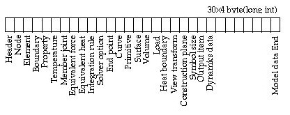
< Modeling data position record>
|
Node: The position of node data. |
|
|
Element: The position of element data. |
|
|
Boundary: The position of structural boundary condition data. |
|
|
Property: The position of element property data. |
|
|
Temperature: The position of temperature data. |
|
|
Member joint: The position of frame member joint data. |
|
|
Equivalent force : The position of equivalent nodal force data. |
|
|
Equivalent heat: The position of equivalent nodal heat data. |
|
|
Integration rule : The position of integration rule record. |
|
|
Solver option : The position of solver option record. |
|
|
End point: The position of curve end point data. |
|
|
Curve: The position of curve data. |
|
|
Primitive: The position of surface primitive data. |
|
|
Surface: The position of surface mesh data. |
|
|
Volume: The position of volume mesh data. |
|
|
Load: The position of load condition data. |
|
|
Heat boundary: The position of heat boundary condition data. |
|
|
View transform: The position of view transformation data. |
|
|
Construction plane: The position of construction plane data. |
|
|
Symbol size: The position of Symbol size record. |
|
|
Output item: The position of output item record. |
|
|
Dynamics data: The position of Dynamics data record. |
|
|
Modeling data end: The position of the end point of the modeling data. |
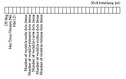
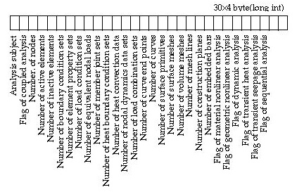
> Header record
Header record has the basic information on the file including the analysis type, sizes of model ingredients, etc. The record has 30 entities of 4 byte long integer. The blank spaces are reserved for future use.
< Header record>
|
Analysis subject: The analysis subject is coded by the following numbers. The analysis subject re p resents the major analysis type which can be mixed with different types of analysis class. (Refer to Chapter 5, "Element Properties".) |
|
0 : plane stress |
|
|
1 : plane strain |
|
|
2 : Axisymmetric |
|
|
3 : plate bending structure |
|
|
4 : shell structure |
|
|
5 : 3 dimensional solid structure |
|
|
6 : 2 dimensional truss |
|
|
7 : 3 dimensional truss |
|
|
8 : 2 dimensional rigid frame |
|
|
9 : 3 dimensional rigid frame |
|
|
10 : plane heat conduction |
|
|
11 : axisymmetric heat conduction |
|
|
12 : 3 dimensional heat conduction |
|
|
13 : plane seepage |
|
|
14 : axisymmetric seepage |
|
|
15 : 3 dimensional seepage |
|
Number of nodes: The total number of nodes in the model |
|
|
Number of active elements: The number of elements used in the finite element analysis. Only elements assigned with element properties are actually included in the analysis. |
|
|
Number of inactive elements: The number of elements without element property assignment. The unassigned elements are not included in the analysis, and thus termed as "inactive element. |
|
|
Number of boundary condition sets: The number of boundary condition sets which include both assigned and unassigned ones. Unassigned set implies the ones defined for user interface, but not yet assigned to any object. |
|
|
Number of element property sets: The number of element property sets which include both assigned and unassigned ones. |
|
|
Number of load condition sets: The number of load condition sets which include both assigned and unassigned ones. |
|
|
Number of equivalent nodal loads: The number of equivalent nodal loads is the same as the number of nodes with non-zero equivalent nodal load. |
|
|
Number of member joint sets: The number of member joint sets which include both assigned and unassigned ones. |
|
|
Number of heat boundary condition sets: The number of heat boundary condition sets which include both assigned and unassigned ones. |
|
|
Number of heat convection data: The number of heat convection data which are extracted from heat boundary condition data. |
|
|
Number of temperature sets: The number of temperature sets which include both assigned and unassigned ones. |
|
|
Number of nodal dynamics data sets: The number of nodal dynamics data sets which include both assigned and unassigned ones. |
|
|
Number of curve end points: The total number of end points which define the starting and ending points of curves. |
|
|
Number of curves: The total number of curves, both created and generated. |
|
|
Number of surface primitives: The total number of surface primitives. |
|
|
Number of surface meshes: The total number of surface meshes, both created and generated. |
|
|
Number of volume meshes: The total number of volume meshes, both created and generated. |
|
|
Number of mesh lines: The total number of straight lines consisting the wireframe meshes. |
|
|
Number of construction planes: The number of construction planes defined for aiding the coordinate data. |
|
|
Flag of nonlinear analysis: The value indicates whether the analysis is linear or nonlinear: 0 for linear analysis and 1 for nonlinear analysis. |
|
|
Flag of dynamic analysis: The value indicates whether the analysis is static or dynamic: 0 for static analysis and 1 for dynamic analysis. |
|
|
Number of frontal buffers: The number of data buffers used in frontal solution process. |
Node data consist of records with nodal coordinates and assignment information, One record contains following information for a node. There are as many records as the number of nodes.
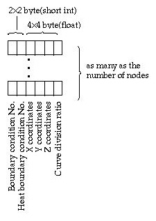
<Node data>
|
Boundary condition No.: The No. of the structural boundary condition set assigned to the node. This value is zero based. (Boundary condition sets are numbered starting from 0.) If this value is -1, the node is not assigned with boundary condition. (2 byte short integer) |
|
|
Heat boundary condition No.: The No. of the heat boundary condition set assigned to the node. This value is zero based. If this value is -1, the node is not assigned with heat boundary condition. (2 byte short integer) |
|
|
X, Y, and Z coordinates: The coordinates of the node in X, Y, Z Cartesian coordinate system. (4 byte float for each one of X, Y and Z coordinates) |
|
|
Curve division ratio: The relative position of the node on the curve. The value is between 0 and 1.0; the node at the starting point of the curve has the value of 0, and the one at the end point of the curve has the value of 1.0. The nodes between the two have the value representing the normalized distance from the starting point. |
|
|
This value has meaning only for the nodes created by dividing curves. This value is not used for solver. This information is used for future modification of the curve. The curve division ratios are retained after modification of curves. (4 byte float) |
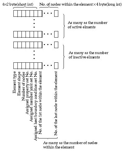
Element data consist of records with nodal connectivities and assignment information. One record contains following information for an element. There are records for active elements followed by the records for inactive elements. Active elements are those actually involved in finite element processing. All the elements
assigned with element properties are active. Inactive elements are not used in the processing, but constitute curve divisions, surface meshes or volume meshes.
VisualFEA represents the segment of curve divisions, surface meshes and volume meshes in the form of element data. These segments become active elements when they are assigned with element properties.
|
Element type: Analysis type of the element. Only active elements have element type. (2 byte short integer) |
||
|
-1 : not an element type (for inactive elements) |
||
|
0 : plane stress |
||
|
1 : plane strain |
||
|
2 : Axisymmetric |
||
|
3 : plate bending structure |
||
|
4 : shell structure |
||
|
5 : 3 dimensional solid structure |
||
|
6 : 2 dimensional truss |
||
|
7 : 3 dimensional truss |
||
|
8 : 2 dimensional rigid frame |
||
|
9 : 3 dimensional rigid frame |
||
|
10 : plane heat conduction |
||
|
11 : axisymmetric heat conduction |
||
|
12 : 3 dimensional heat conduction |
||
|
16 : interface element |
||
|
17 : embedded bar |
||
|
Element shape: The shape of the element (2 byte short integer) |
||
|
1 : 2 node line element |
||
|
2 : 3 node line element |
||
|
3 : 3 node triangular element |
||
|
4 : 6 node triangular element |
||
|
5 : 4 node quadrilateral element |
||
|
6 : 8 node quadrilateral element |
||
|
7 : 4 node tetrahedral element |
||
|
8 : 10 node tetrahedral element |
||
|
9 : 6 node prism element |
||
|
10 : 15 node prism element |
||
|
11 : 8 node hexahedral element |
||
|
12 : 20 node hexahedral element |
||
|
<Element data> |
||
|
Number of nodes: The number of nodes in the element. (2 byte short integer) |
||
|
Assigned property set No.: The zero based No. of the element property set assigned to the element. If this value is -1, the element is not assigned with element property set. (2 byte short integer) |
||
|
Assigned member joint set No.: The zero based No. of the member joint set assigned to the element. If this value is -1, the element is not assigned with member joint set. (2 byte short integer) |
||
|
Assigned heat boundary condition set No.: The zero based No. of the heat boundary condition set assigned to the element. If this value is -1, the element is not assigned with heat boundary condition set. (2 byte short integer) |
||
|
Node No.: The zero based No. of each node within the element. (number of nodes within the element 4 byte long integer ) |
||
The boundary condition data consist of records with structural fixities and either initial displacements or spring constants of the node. One record contains information for one boundary condition set as follows.
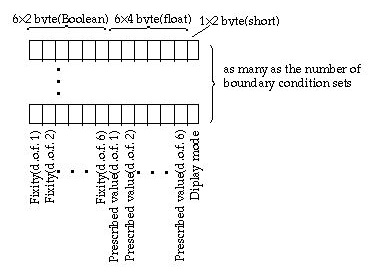
<Boundary condition data>
|
Fixity: Structural fixity or restraint of each nodal d.o.f. at a node. There are 6 entries of fixity data, but only the entries corresponding to the actual nodal d.o.f. are in use. (6 2 byte short integer) |
||
|
0 : fixed |
||
|
1 : free |
||
|
Prescribed value: Value prescribed for each nodal d.o.f. at a node. There are 6 entries of prescribed values, but only the entries corresponding to the actual nodal d.o.f. are in use. The prescribed values are either initial displacements or spring constants. If the nodal d.o.f. is fixed, the prescribed value represent the initial displacement of the corresponding d.o.f. Otherwise, the value represents the spring constant assigned to the corresponding d.o.f. (6 4 byte float) |
||
|
Display mode: mode of displaying the prescribed values on "Struct Boundary" dialog. (Refer to Chapter 5) The edit text items of initial displacement, spring constant or both are displayed on the dialog depending on the mode. |
||
|
0 : Only edit text boxes of initial displacements are displayed. |
||
|
1 : Only edit text boxes of spring constants are displayed. |
||
|
2 : All edit text boxes are displayed. |
||
The element property data have a variable number of data items. The number of data items and the entity of each item are determined by the element type defined for the set, and appear on "Property" dialog.
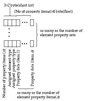
<Element property data>
|
Number of property items: The number of element property items are variable, and retrieved by this entry. This value is originally determined by the element type at the stage of pre p rocessing, but saved and retrieved as an entry of element property data for quick retrieval of the data items. (2 byte short integer) |
||
|
Assigned element type: The element type is primarily determined by the analysis type. However, VisualFEA allows mixed use of diff e rent element types in a model. (2 byte short integer) |
||
|
-1 : not an element type (for inactive elements) |
||
|
0 : plane stress |
||
|
1 : plane strain |
||
|
2 : Axisymmetric |
||
|
3 : plate bending structure |
||
|
4 : shell structure |
||
|
5 : 3 dimensional solid structure |
||
|
6 : 2 dimensional truss |
||
|
7 : 3 dimensional truss |
||
|
8 : 2 dimensional rigid frame |
||
|
9 : 3 dimensional rigid frame |
||
|
10 : plane heat conduction |
||
|
11 : axisymmetric heat conduction |
||
|
12 : 3 dimensional heat conduction |
||
|
13 : plane seepage |
||
|
14: axisymmetric seepage |
||
|
15 : 3 dimensional seepage |
||
|
16 : interface element |
||
|
17 : slip bar |
||
|
18 : embedded bar |
||
|
Assigned property type: The type of material property (2 byte short integer) |
||
|
0 : linear elastic and isotropic |
||
|
1 : linear elastic and orthotropic |
||
|
2 : elasto-plastic( appears only for nonlinear analysis) |
||
|
3 : friction( appears only for interface elements of nonlinear analysis) |
||
|
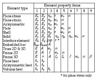
Property data items: The number of data items is retrieved as an entry of a data record, and the entity of each item is determined by the element type as shown in the following table. (number of data items 4 byte float) |
||
|
<Entities of element property items>
* for plane stress only |
In case the element type is embedded bar, one more data item is added as shown below. The additional item points to the set No. of the property surrounding the embedded bar.
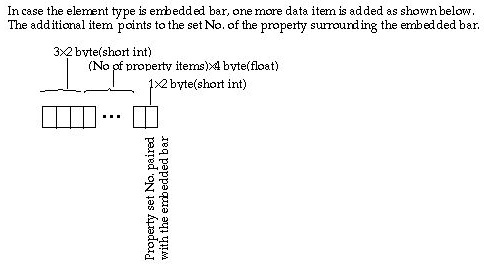
<Element property data for embedded bar>
> Temperature data
Temperature data are currently applicable only to 2-D and 3-D frame analysis. The data consist of the average temperature of a frame member and the temperature gradient across the member section.
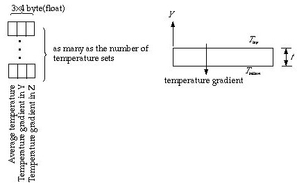
<Temperature data>
|
Average temperature: Average temperature of the frame member(4 byte float) |
|
|
Temperature gradient in Y: Temperature gradient across the member section in Y direction. The gradient is equivalent to the temperature difference between top and bottom of the section divided by the height of the section. (4 byte float) |
|
|
Temperature gradient in Z: Temperature gradient across the member section in Z direction. This item is used only for 3-D frames. (4 byte float) |
|
|
Temperature data are not supported by user interface in the current version of VisualFEA. Instead, they are treated as thermal load conditions. Refer to Chapter 5. However, their space is left in VisualFEA file for use by external software. |
Member joint data are currently applicable to 2-D and 3-D frame analysis. One record of member joint data has only 2 data items: joint states at both end of the member.
|
Joint state (left node): The state of joint at the starting point of the member. (2 byte short int) |
||
|
0 : Rigid joint |
||
|
1 : Pin joint |
||
|
Joint state (right node): The state of joint at the ending point of the member. (2 byte short int) |
||
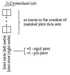
<Member joint data>
The equivalent nodal forces are computed at each node from the load condition data, which is described in one of the later sections. The equivalent nodal forces are directly involved in finite element analysis, while the load condition data are maintained chiefly for graphical user interface. The data has records only for nodes with non-zero equivalent nodal forces. The components of the equivalent nodal forces are as many as the number of nodal d.o.f.
|
Node No.: The node No. identifying the node for which the equivalent nodal forces are evaluated. (4 byte long int) |
|
|
Equivalent nodal force magnitude: Magnitude of each force component which matches with each one of the nodal d.o.f. (number of nodal d.o.f. 4 byte float) |
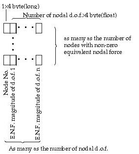
<Equivalent nodal force data>
This data portion consists of two parts: equivalent nodal heat and convection boundary condition data. Both parts are evaluated from heat boundary condition data. The equivalent nodal heat data has records for all nodes in the model. Each record has only 2 data entries:
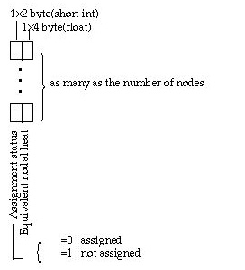
<Equivalent nodal heat data>
|
Assignment status: Flag indicating whether the node is assigned with nodal heat. (2 byte short int) |
||
|
0 : Assigned |
||
|
1 : Not assigned |
||
|
Equivalent nodal heat: Magnitude of nodal heat (4 byte float) |
||
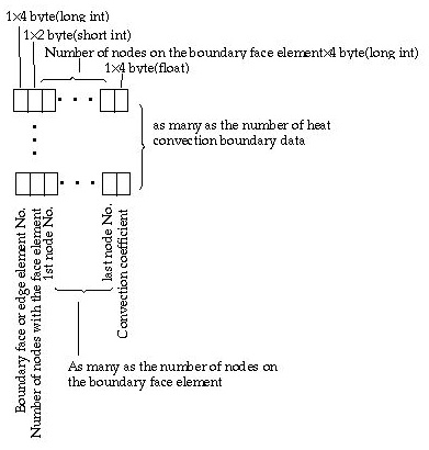
In the second part are the convection boundary condition data, which are evaluated from convection type of heat boundary condition. The data consist of convection coefficients and information on boundary face or edge on which the convection boundary condition is applied.
|
Boundary face or edge element No.: The convection boundary conditions are applied to the inactive elements on boundary edges (2-D case) or on boundary faces (3-D case). This data entry has the element No. on the boundary edge or face. (4 byte long int) |
|
|
Number of nodes within the face or edge element: The face or edge consists of a number of nodes. This entry has the number of nodes within the element. (4 byte long int) |
|
|
Node No.: All the node No. consisting the boundary face or edge element. (number of nodes within the boundary element 4 byte long int) |
|
|
Convection coefficient: The convection coefficient of the heat boundary condition set from which the equivalent nodal heat is evaluated. (4 byte float) |
|
|
<Convection boundary data> |
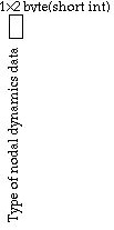
The number of nodal dynamics data sets is included in the data header record, and is always zero for static analysis. The following represents only one set of nodal dynamics data records. These data records occur as many times as the number of nodal dynamics data sets. Each set of data records starts with an attribute classifying the type of nodal dynamics data.
|
Type of nodal dynamics data: This data entry represent the type of nodal dynamics data as follows: |
||
|
1 : Nodal dynamic motion - displacement |
||
|
2 : Nodal dynamic motion - velocity |
||
|
3 : Nodal dynamic motion - acceleration |
||
|
4 : Nodal dashpot constant |
||
|
5 : Nodal mass |
The contents for the rest of the nodal dynamics data records are different depending on the type of nodal dynamics data. In case of nodal dashpot and nodal mass, the data consist of 6 entries which represent the values for each nodal d.o.f.
<Attribute classifying the type of nodal dynamics data>
The integration scheme is set independently for each shape and each order of element. The number of integration points set for various element shapes are saved in the integration scheme data record as shown in the following figure . There are 30 entries of 4 byte long integer in the record. The blank spaces are reserve for future use.
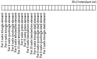
<Integration scheme record>
|
For 3 node triangle element: Number of integration points set for a 3 node triangle element. It is either of 1, 3 or 7. |
|
|
For 6 node triangle element: Number of integration points set for a 6 node triangle element. It is either of 1, 3 or 7. |
|
|
For 4 node quadrangle element: Number of integration points set for a 4 node quadrangle element. It is either of 1, 4 or 9. |
|
|
For 8 node quadrangle element: Number of integration points set for a 8 node quadrangle element. It is either of 1, 4 or 9. |
|
|
For 4 node tetrahedron element: Number of integration points set for a 4 node tetrahedron element. It is either of 1, 4 or 5. |
|
|
For 10 node tetrahedron element: Number of integration points set for a 10 node tetrahedron element. It is either of 1, 4 or 5. |
|
|
For 6 node prism element: Number of integration points set for a 6 node prism element. It is either of 1, 2or 6. |
|
|
For 15 node prism element: Number of integration points set for a 15 node prism element. It is either of 1, 2or 6. |
|
|
For 8 node hexahedron element: Number of integration points set for a 8 node hexahedron element. It is either of 1, 8or 27. |
|
|
For 20 node hexahedron element: Number of integration points set for a 20 node hexahedron element. It is either of 1, 8or 27. |
> Solver option record
There are a number of options which are applied for finite element processing. They are saved in the solver option record with 30 entries of 2 byte short integer. Each entry has value of 0 or 1. The option is on if the value is 1 and off otherwise, except the equation solver option.
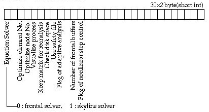
<Solver option record>
|
Equation solver: One of skyline solver and frontal solver is selected as the equation solver. |
||
|
0 : Frontal solver |
||
|
1 : Skyline solver |
||
|
Optimize element No.: Element number optimization is executed before finite element processing begins, if this option is on. |
||
|
Optimize node No.: Node number optimization is executed before finite element processing begins, if this option is on. |
||
|
Visualize process: The pro g ress of finite element processing is graphically visualized, if this option is on. |
||
|
Keep matrix for reanalysis: The relevant matrix files necessary for reanalysis are not removed at the end of the processing, if this option is on. |
||
|
Check disk space: The available disk space is continuously checked while the processing is going on, if this option is on. |
||
|
Use safety file: A temporary file is created and used while processing is going on, in order to protect the original file from being damaged under abnormal situation, if this option is on. |
||
|
Flag adaptive analysis: An iterative analysis process with adaptive mesh generation is applied if this option is on. |
||
|
Number of frontal buffer: This entry specifies the number of matrix data used for frontal solver. |
||
|
Flag of nonlinear step control: If this flag is on, the rate load increment is specified individually for each of the load step. |
||
> Analysis output item record
Each entry has value of 0 or 1. If the value is 1, corresponding item is turned on as an analysis output item. There are 30 entries of 2 byte short integer in the record. The blank spaces are reserved for future use.
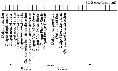
<Analysis output item record>
|
Output reaction - output heat flux direction: The corresponding data are computed and saved as part of analysis data, if the respective option is on. |
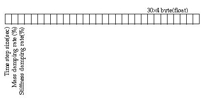
> Dynamic analysis setting record
There are a few options and variables for dynamic analysis. They consist of 2 records, one with integer data entries and the other with floating point data entries.
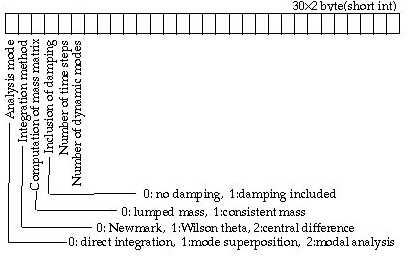
<Dynamic analysis setting record 1>
|
Analysis mode : This entry re p resent mode of dynamic analysis, direct integration, mode superposition, and modal analysis. |
|
|
Integration method : data designating one of the 4 different methods of integration for dynamic analysis. |
|
|
Computation of mass matrix : This entry indicates whether lumped mass or consistent mass is assumed for mass matrix computation. |
|
|
Inclusion of damping : This entry indicates whether damping is included in the dynamic analysis. |
|
|
Number of time step : The number of time steps included in the analysis. This entry is ignored in modal analysis. |
|
|
Number of dynamic modes : The number of modes computed and used for analysis. This entry is ignored in direct integration. |
|
|
<Dynamic analysis setting record 2> |
|
|
Time step size : The interval from one time step to the next. Uniform size is assumed for all time steps. |
|
|
Mass damping rate(%) : The damping ratio applied for mass. |
|
|
Stiffness damping rate(%) : The damping ratio applied for stiffness. |
> Curve end point data
Every curve has two end points, a starting point and a ending point. The coordinates of these end points are saved as curve end point data.
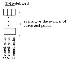
<Curve end point data>
X, Y, and Z coordinates: The coordinates of the end point in X, Y, Z Cartesian coordinate system. (4 byte float for each one of X, Y and Z coordinates)
> Curve data
A curve exists either as a single entity or as multiple entities linked together. The curve data are generalized in the form of linked curve as shown in the following figure.
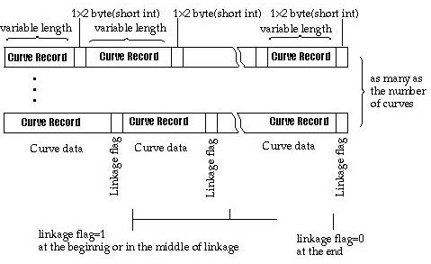
<Linked curve data>
|
Curve record: A curve record has information on a single curve as described below. (variable length) |
||
| linkage flag: flag indicating if the curve is linked at the end. (2 byte short int) | ||
| 0 : No further linkage at the end. The flag is always 0 at the end of linked curves. | ||
| 1 : curve linked at the end. The flag is always 1 in the middle of linked curves. | ||
A curve re c o rd contains information on the geometric composition and the attribute assignment, and other characteristics of a single curve. A curve is composed of end points, control points, nodes and elements.
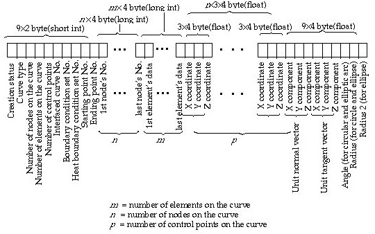
<Curve record>
|
Creation status: A curve may be either created by user interaction inputting control points, or generated in the process of finite element mesh generation. The boundary of surface meshes are always defined by curves. The creation status indicates whether the curve was created or generated. (2 byte integer) |
||
|
0 : Generated. |
||
|
1 : Created |
||
|
Curve type: This value represent the type of the curve as follows. |
||
|
-1 : Not a valid curve. |
||
|
0 : Point |
||
|
1 : Straight line |
||
|
10 : Acute arc |
||
|
11 : Clockwise arc |
||
|
12 : Counter clockwise arc |
||
|
13 : Three point arc |
||
|
14 : Center angle arc |
||
|
16 : Clockwise circle |
||
|
17 : Counter clockwise circle |
||
|
18 : Three point circle |
||
|
19 : Center radius circle |
||
|
21 : Quarter ellipse |
||
|
22 : Half ellipse |
||
|
23 : Full ellipse |
||
|
31 : Cubic spline curve |
||
|
32 : B-spline curve |
||
|
33 : Bezier curve |
||
|
34 : Polynomial curve |
||
|
35 : Polyline |
||
|
36 : Segmented curve |
||
|
41 : Rectangle |
||
|
Number of nodes on the curve: The number of nodes which were created by dividing the curve, or generated together with the curve. |
||
|
Number of elements on the curve: The number of elements which were created by dividing the curve, or generated together with the curve. |
||
|
Number of control points on the curve: The number of control points which define the geometry of the curve. |
||
|
Interface curve No.: When interface elements are assigned along the curve, a duplicate of the curve is generated to form another boundary of the interface gap. In this case, this entry has the pairing interface curve No. |
||
|
Boundary condition set No.: If the curve is assigned with a boundary condition, this entry has its No. which is zero based. If boundary condition is not assigned, the value is -1. |
||
|
Heat boundary condition set No.: If the curve is assigned with a heat boundary condition, this entry has its No. which is zero based. If heat boundary condition is not assigned, the value is -1. |
||
|
Starting point No.: The No. of the end point serving as the starting point of the curve. |
||
|
Ending point No.: The No. of the end point serving as the ending point of the curve. |
||
|
Node No.: The No. of each node on the curve. This value is zero based. In other words, the node No. starts from 0. |
||
|
Element No.: The No. of each element on the curve. This value is zero based. In other words, the element No. starts from 0. |
||
|
Coordinates of control points: X, Y and Z coordinates of control points on the curve. Z value is zero for 2 dimensional case. |
||
|
Unit normal vector: This entry applies only to circular arc, circle, elliptical arc and ellipse. The directional cosines of the unit normal vector to the curve are saved respectively in X, Y and Z components. |
||
|
Unit tangent vector: This entry applies only to closed cubic spline, B-spline or Bezier curves. The unit tangent vector is tangent to the curve at the starting or the ending point. The directional cosines of this unit tangent vector are saved respectively in X, Y and Z component. |
||
|
Angle : This entry applies only to circular arc and elliptical arc. Angle implies the central angle of the curve. |
||
|
Radius: This entry applies only to circle and ellipse. This is the radius of a circle, and first radius of an ellipse. |
||
|
Radius 2: This entry applies only to ellipse. This is the second radius of an ellipse. |
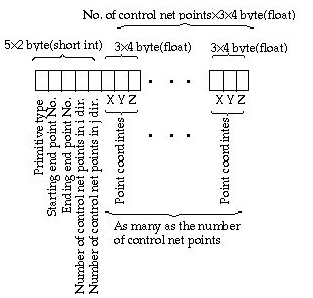
> Primitive surface data
Primitive surface data consists of primitive records. Of course, there are as many records as the number of primitive surfaces. The records have two different compositions depending on the type of the primitives. The primitive record of sphere, cylinder, and torus is one kind, and that of plane, Lagrangian surface, Bspline surface and Bezier surface is another kind. The primitive record for the first kind is shown in the following figure.
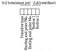
<Primitive record for sphere, cylinder and torus>
|
Primitive type: This entry has the code indicating the type of the primitive. |
||
|
82 : Sphere |
||
|
83 : Cylinder |
||
|
84 : Torus |
||
|
Starting end point No.: The No. of the end point serving as the starting point of the primitive. |
||
|
Ending end point No.: The No. of the end point serving as the ending point of the primitive. |
||
|
Radius 1: The first radius of the primitive surface |
||
|
Radius 2: The second radius of the primitive surface. Sphere has only one radius, thus this value is ignored in sphere data. |
||
|
<Primitive record for plane, Lagrangian, B-spline and Bezier surfaces> |
||
|
Primitive type: The type of the primitive |
||
|
85 : B-spline surface |
||
|
86: Bezier surface |
||
|
87 : Lagrangian surface |
||
|
Starting end point No.: The No. of the end point serving as the starting point of the primitive. |
||
|
Ending end point No.: The No. of the end point serving as the ending point of the primitive. |
||
|
Number of control net points in i direction: The primitive surface is defined by m x n control net points where m and n represent the number of control points in i and j direction. This entry has the value of m. |
||
|
Number of control net points in j direction: This entry has the value of n. |
||
|
Control net point coordinates: The X, Y, and Z coordinates of each of m x n control net points. |
||
> Surface mesh data
Surface data have the information on the surface meshes including their compositions, attribute assignments, and other characteristics.
A surface mesh is composed of nodes, elements, wireframe lines and boundary curves. Information on the nodes on the surface can be derived from that of the elements on the surface. And therefore, information on the nodes are not included in the surface data.
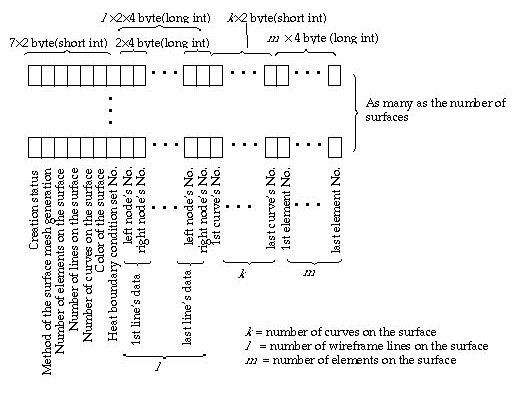
<Surface data>
|
Creation status: A surface mesh may be either created by user interaction using surface mesh generation command, or generated in the process of volume mesh generation. The boundary of volume meshes are always defined by surface meshes. The creation status indicates whether the surface mesh was created or generated. |
||
|
0 : Generated. |
||
|
1 : Created |
||
|
Method of surface mesh generation: The entry has the code representing the method of surface mesh generation which was applied to create the surface. |
||
|
0 : Surface mesh generation by 2 edge mapping |
||
|
1: Surface mesh generation by extrusion |
||
|
2: Surface mesh generation by 4 edge mapping |
||
|
3: Surface mesh generation by 3 edge mapping |
||
|
4: Surface mesh generation by revolution |
||
|
5: Surface mesh generation by translation |
||
|
12: Surface mesh generation by automatic triangulation |
||
|
13: Surface mesh generation by automatic tetrahedronization |
||
|
14: Volume mesh generation by duplication with "Move" |
||
|
15: Surface mesh generation by duplication with "Move" |
||
|
18: Surface mesh generation by duplication with "Revolve" |
||
|
21: Surface mesh generation by duplication with "Mirror" |
||
|
24: Surface mesh generation by twisting |
||
|
28: Surface mesh generation by duplication with "Extrude" |
||
|
29: Surface mesh generation by projection |
||
|
Number of elements on the surface: Number of all elements, either active or inactive, composing the surface. |
||
|
Number of lines on the surface: Number of all lines re p resenting the wireframe of the surface mesh. |
||
|
Number of curves on the surface: Number of all curves attached to the surface. |
||
|
Color of the surface: The color assigned to the surface. (currently not in use, but reserved for future use) |
||
|
Heat boundary condition set No.: No. of the heat boundary condition set assigned to the surface. |
||
|
Line data: Information on the lines forming the wireframe. A line is represented by two end nodes. Thus, the data for a line consist of 2 entries; the 2 end node's No. |
||
|
Curve No.: The No. of each curve in the surface mesh. |
||
|
Element No.: The No. of each element in the surface mesh. |
> Volume mesh data
Volume data have the information on the volume meshes including their compositions, attribute assignments, and other characteristics.
A surface mesh is composed of nodes, elements, surface meshes. Information on the nodes on the volume can be derived from that of the elements on the volume. And therefore , information on the nodes are not included in the volume data.
|
Creation status: Not used in the current version. Reserved for future use. |
||
|
Method of volume mesh generation: The entry has the code representing the method of volume mesh generation which was applied to create the volume. |
||
|
6: Volume mesh generation by 2 surface mapping |
||
|
7: Volume mesh generation by extrusion |
||
|
8: Volume mesh generation by box edge mapping |
||
|
9: Volume mesh generation by tetrahedron edge mapping |
||
|
9: Volume mesh generation by revolution |
||
|
10: Volume mesh generation by translation |
||
|
17: Volume mesh generation by duplication with "Revolve" |
||
|
20: Volume mesh generation by duplication with "Mirror" |
||
|
27: Volume mesh generation by prism edge mapping |
||
|
23: Volume mesh generation by twisting |
||
|
Number of surfaces on the volume : The number of surfaces attached to the volume. The boundary surface of a volume is composed of surface meshes. |
||
|
Color of the volume : Code of the color assigned to the volume. This entry is not used in the current version, but reserved for future use. |
||
|
Heat boundary condition set No.: No. of the heat boundary condition set assigned to the volume mesh. |
||
|
Number of elements in the volume: Number of all elements, either active or inactive, composing the volume mesh. |
||
|
Surface No.: The No. of each surface in the volume mesh. |
||
| Element No.: The No. of each element in the volume mesh. |
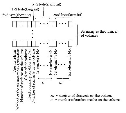
<Volume data>
> Load condition data - header record
These data are maintained chiefly for graphical user interface, and involved indirectly, through equivalent nodal forces, in finite element analysis. They are also the source from which the equivalent nodal forces are computed. The contents of load conditions vary depending on their type as described below.
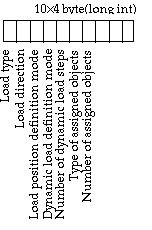
< Load condition data >
|
Load type: The code representing the type of the load. |
||
|
0: Nodal force |
||
|
1: Point force |
||
|
2: Uniform force |
||
|
3: Non-uniform force with linear variation |
||
|
4: Non-uniform force with parabolic variation |
||
|
5: Bilinear force |
||
|
6: Nodal moment |
||
|
7: Point moment |
||
|
8: Uniform moment |
||
|
9: Body force |
||
|
10: Hydrostatic in X |
||
|
11: Hydrostatic in Y |
||
|
12: Hydrostatic in Z |
||
|
13: Self straining force |
||
|
14: Thermal force |
||
|
Load direction: The code representing the direction of the load. |
||
|
0: X direction |
||
|
1: Y direction |
||
|
2: Z direction |
||
|
3: Direction normal to curve |
||
|
4: Direction tangent to curve |
||
|
5: Direction normal to surface |
||
|
6: Direction tangent to surface and normal to X direction |
||
|
7: Direction tangent to surface and normal to Y direction |
||
|
8: Direction tangent to surface and normal to Z direction |
||
|
Load position definition mode: This entry designates how the position of the load is defined. This applies only to mid-point force or mid-point moment, and is ignored for other load types. The position of mid-point force or moment can be defined either by the actual distance from one end of the structural member, or by the relative distance represented by the ratio to the length of the member. Distance ratio is equivalent to the distance divided by the total length of the member. The load position definition mode can applied also for a curve instead of a member. |
||
|
0: Actual distance |
||
|
1: Relative distance |
||
|
Dynamic load definition mode: Time dependent dynamic loads can be defined either as a sinusoidal harmonic load or as a transient load. |
||
|
0: Harmonic load |
||
|
1: Transient load |
||
|
Number of dynamic load steps: The number of steps re p resenting the dynamic load history. This data entry is effective only for transient load, and ignored for static loads or harmonic loads. |
||
|
Type of assigned objects: The type of the object to which the load condition is assigned. |
||
|
-1: Not assigned |
||
|
1: Curve |
||
|
2: Surface |
||
|
3: Volume |
||
|
4: Element |
||
|
5: Node |
||
|
7: Surface primitive |
||
|
11: Line element |
||
|
12: Surface element |
||
|
13: Volume element |
||
|
Number of assigned objects: The type of the object to which the load condition is assigned. |
||
> Load condition data - attribute record
This data record consists of load attributes such as its magnitude, position and etc. Only one of the following 3 records is applied depending on whether the load is static, dynamic transient, or dynamic harmonic,

< Load attribute record for a static load>
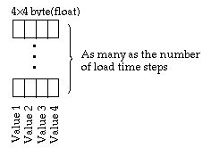
< Load attribute record for a transient load>
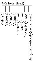
< Load attribute record for a harmonic load >
|
Value 1, Value 2, Value 3, Value 4: These entries are data entered using the editable text items of "Load Condition" dialog. Their contents vary depending on the load type as shown below. Also refer to Chapter 5. |
|
|
Starting time: The time from which the harmonic load becomes effective. |
|
|
Ending time: The time when the harmonic load ends. |
|
|
Phase lag time(to): Phase lag to the starting point of the sinusoidal loading curve. |
|
| Angular velocity(w): Radian per second. |
A harmonic load is defined by the following sine wave form The amplitude of the load is given by value 1, 2, 3 or 4 in the load attribute record.
<Contents of load condition values>
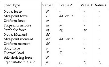
For bilinear force, the coordinates of the 4 corner points defining the distribution of the load should be supplied in addition as follows.
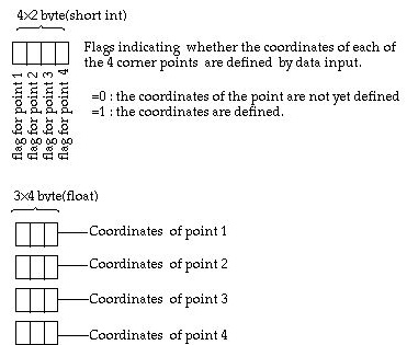
<Coordinates of 4 corner points of bilinear force>
> Load condition data - assigned objects
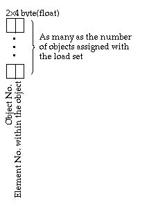
|
Object No.: The No. of the object to which the load condition is assigned. Or, if the object type is "Element" this entry has the No. of the object to which the element belongs. |
|
| Element No. within the object: The No. of the element within the object. This entry is used, only in case the Object type is element. |
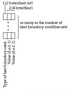
> Heat boundary condition data
The heat boundary condition data are maintained chiefly for graphical user interface, and involved indirectly, through equivalent nodal heat and convection boundary conditions, in finite element analysis. They are also the source fro m which the equivalent nodal heats and convection boundary conditions are computed. The items of heat boundary conditions vary depending on their type as described below.
<Heat boundary condition data>
|
Heat boundary condition type: The code re p resenting the type of the heat boundary condition. |
||
|
0: Temperature |
||
|
1: Convection |
||
|
2: Heat flux |
||
|
3: Point source |
||
|
4: Element source |
||
|
5: Region source |
||
|
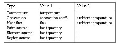
Value 1 - 4: These entries are data entered using the editable text items of "Heat Boundary" dialog. Their contents vary depending on the type of the heat boundary condition as shown below. Also refer to Chapter 5. |
||
<Contents of load condition values>
> View transformation data
View transform data consists of information on grid setting and view transformation in interactive work environment, the state of which at the time of file saving is retrieved and applied as the initial setting when the file opened. The view transformation data may be saved in an independent view files, if necessary. The record contains the same contents both for a VisualFEA file and for an independent view file.
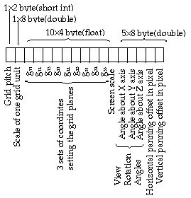
< View transformation data>
|
Grid pitch : Number of pixels between grid lines on the screen with initial view transformation. This is the value entered "Grid Setting" dialog, or "Rreference" dialog as described in Chapter 2. |
||
|
Grid scale : The actual distance re p resented by the interval between two adjacent grid lines. This value is also entered using "Grid Setting" dialog, or "Rreference" dialog. |
||
|
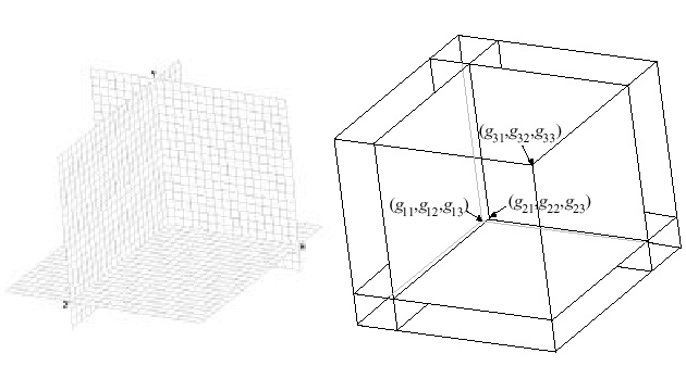
Grid box coordinates : 3 sets of XYZ coordinates setting the planes as shown in the figure below. These values are inputted by interactively moving or resizing the grid planes as explained in Chapter 2. |
||
|
Screen scale : Zoom factor inputted by interactive view scaling action as explained in Chapter 2. The view scale, which is the ratio between the screen coordinates in pixels and the actual coordinates, are determined by |
||
| view scale = grid pitch x grid scale x screen scale | ||
|
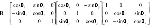
View rotation angles : Angles of view rotation about X, Y and Z axes respectively. These angles are used in computing the view rotation matrix R by the following equation. |
||
|
< Grid box coordinates>
|
||
|
Horizontal panning offset : Horizontal offset distance of screen view in pixels. This value is changed by panning the screen view in horizontal direction as described in Chapter 2. |
||
|
Vertical panning offset : Vertical offset distance of screen view in pixels. This value is changed by panning the screen view in vertical direction as described in Chapter 2. |
> Construction plane data
Construction plane is a user defined grid plane with grid points for coordinate input. They are created interactively as described in Chapter 2. A plane in 3 dimensional space is uniquely defined by 3 points on the plane. The planes are not usually parallel to X, Y or Z axis. Their orientation is saved in a 3×3 dtransformation matrix. Each construction plane has its own name which is saved as a character string. The length of the name is variable. The construction plane data have as many records as the number of construction planes which is contained in the header record. Refer to Chapter 2 for creation and use of user defined grid plane.
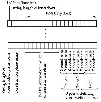
< Construction plane data>
|
String length of construction plane name : The number of characters used for the construction plane name. |
|
|
Construction plane name: Character string of the construction plane name. The name is endowed at the time of creating the construction plane. And this name is used to retrieve the construction plane. |
|
|
Transformation matrix of construction plane: 3 3 matrix setting the orientation of the construction plane. |
|
|
Coordinates of 3 points defining the construction plane: X, Y and Z coordinates of 3 points which were inputted in order to define the plane. |
> Symbol size record
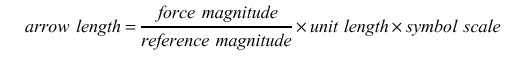
A force of a load condition is symbolized by an arrow. The length of the arrow is drawn approximately in proportion to the length of the force magnitude. The proportion can be set differently for various load types. It is also possible to set the reference magnitude of the force for unit length of the arrow differently for various load types. The force types are classified differently from the actual types used in load condition data. They are point load, curve force, surface, volume force, point moment, curve moment, self straining force and thermal force. The line length of the arrow in pixels is computed as follows:
|
Symbol scale : One symbol scale for each one of the load types, |
|
| Reference magnitude: One reference magnitude for each one of the load |
< Symbol size record>
|
|
|
|