Visual Instruction of Shape Function and Interpolation

Understanding the characteristics of a shape function

In general, the shape function of an element is determined by the shape, the order (or number of nodes), and the analysis type (plane stress, plate bending, etc.) of the element. Conergene of the finite element solution is closely related to the characteristics of the shape function employed in the element modeling. This educational function of VisualFEA/CBT is useful for visual instruction and understanding of various shape functions and their characteristics. Especially, their behaviors can be studied in conjunction with the convergence requirements of a finite element solution.

Comparing shape functions of different element shape and order

VisualFEA/CBT can display the shape function of the following elements only.

In order to facilitate comparison between shape functions of the above elements, it is desirable to create a simple model which includes all of those elements as exemplified below. Such a simple finite element model is also useful for examining the continuity of shape function which is described in the later part of this section.

< A simple finite element model created for comparison of shape functions >

The shape functions may be compared for each individual element or for a group of adjacent elements. The interpolation model for a group of adjacent elements may be formed either with elements of identical shape and order, or with a mixture of elements with different shapes and orders.

<Comparison of shape functions for different element shapes and orders>

Understanding the behavior of the shape function gradients

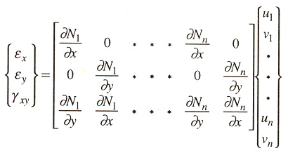
This educational function helps in explaining or understanding the behavior of the shape function gradients (or derivatives), from which strains or heat fluxes are computed. In plane stress and strain cases, for example, we can easily associate the shape function derivatives with the strains, as represented by the expression,

where | e_x e_y g_xy | and | u₁ v₁ · · · u_n v_n | represent strain vector and nodal displacement vector respectively.

Examining the geometry of an isoparametric element

In an isoparametric element, geometry is defined by the same shape functions as those for interpolating the behavior of the element. That is,

where the index i is for each node within the element, and the Ni a re the same shape functions as used to interpolate the field quantity D. As expressed by the equation, the coordinate x of an arbitrary point within the element is defined by interpolating the nodal coordinates xi. Therefore, an edge of a quadratic element, for example, is defined by a quadratic curve. The example shown in the figure below can be made by the following steps:

The isopaametrc interpolation of the geometry can be identified by the curved shape of the wireframe model on “Shape Function” window. It is the geometry of the element actually used in finite element modeling. By moving the node in Z direction using key board input in “Node Info” dialog, the element shape can be made the same as obtained from the interpolation of the nodal value.

< A Shape function and its derivates for 4 node quadrilateral element>

Examining C⁰ continuity of the interpolation model

Continuity of the shape function within an element or across element boundaries is one of the required element properties for proper convergence of finite element solution. Continuity of the shape function or interpolated value itself is called C⁰ contuity. For plane stress/strain, axisymmetric, and 3-D solid modeling, this continuity is the one necessary and sufficient for convergence.

C⁰ continuity across the element boundaries can be examined by forming an interpolation model with a few adjacent elements and displaying the interpolated value. The figure below shows examples of inter-element continuity of isoparametric shape functions plane stress/strain and axisymmetric modeling.

This example shows 3 different cases as follows:

< Example of interpolation model for plane elasticity >

Examining C¹ continuity of the interpolation model

Continuity in the first derivatives of the shape function or interpolated value is called C¹ continuity. Some finite elements, such as thin plate or shell elements, are enforced with C¹ contiuiy, and thus called C¹ elements. Hermite polynomials can be used for interpolation of C¹ elements. Hermite interpolation for a 4 node rectangle element is expressed by the equation

where Ni₀, N_ix, N_iy and N_ixy a re the interpolation functions formed by Hermite polynomials. The cross derivative ¶ D / ¶_x¶y is not used as a nodal d.o.f. in the current version of VisualFEA/CBT. Accordingly, it is assumed that values of is zero at all nodes.

The following steps should be taken to examine C¹ continuity.

	1) Define problem type as “Plate bending”.
		Choose “New” or “Problem Setup...” item from menu. Then, “Problem Setup” dialog appears. Click “Plate bending” radio button.
	2) Create a number of 4 node rectangular plate bending elements.
		Define 4 straight lines in rectangle form, divide them properly, and generate mesh based on these curves. It is good to use “4 Edges” scheme.
	3) Assign element properties to the model.
		The type of element is completely defined by assigning the element property.
	4) Choose “Shape Function” item from “Stiffness” submenu of menu.
		“Shape Function” window appears on the screen, and “Interpolate” menu is attached to the menu bar.
	5) Form an interpolation model with two or more adjacent elements.
		Select two or more adjacent elements using rubber-band rectangle, or option click. The selected elements appear on “Shape Function” window.
	6) Transform the view of the interpolation model.
		Rotate, zoom and pan the view of the interpolation model in “Shape Function” window so that the model can be viewed properly.
	7) Assign the nodal values to the interpolation model.
		Not only the nodal values but also their 1st derivatives are interpolated for C1 elements. Therefore, the nodal values and their derivatives should be assigned to the interpolation model. The nodal values can be assigned by dragging the nodes as in case of C0 element. Their derivatives ¶D/ ¶ xand ¶D/ ¶ y can be assigned using handles attached on each node.

< Assigning nodal value and derivatives to C¹ elements >

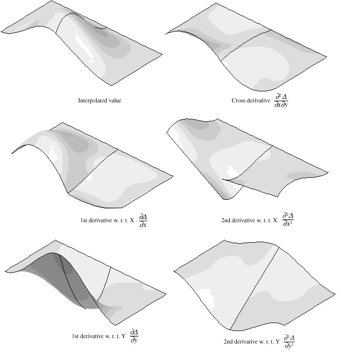
For the above deformation state, the interpolated values and their derivatives displayed as shown in the figure below, by choosing the corresponding menu items from menu. The continuity of the interpolation model is clearly illustrated in the figure. The interpolated value itself is continuous across the element boundary. The first derivatives ¶D / ¶x and ¶D / ¶y, and the cross derivative ¶² D / ¶x ¶y are also continuous at the element boundary. But, the second derivative w.r.t. X ¶²D / ¶x² is not continuous. Although the second derivative w.r.t. Y ¶²D / ¶ y² is appears to be continuous , this is not the general case. It is continuous for this model only because the boundary is parallel to Y axis.

Otherwise, it is not continuous at the boundary either. It is explained in this example that the interpolation model with Hermite polynomials is C¹ continuous. However, it should be noted that the C⁰ continuity is guaranteed only for rectangular elements. The continuity of ¶D / ¶x, ¶D /¶y and ¶²D / ¶x¶y may or may not be preserved for 4-node quadrilaterals other than rectangle, depending on the orientation of the element and the continuity of its edge direction across an adjacent element. It is worth while to examine the continuity of interpolation model under various combination of adjacent elements.

< Continuity of Hermite interpolation model >