![]()
![]()
![]()
![]()
| Basic User Interface > Project and File > Setting preferences |
|
|
|
|
||
Setting preferences
> Grid settings
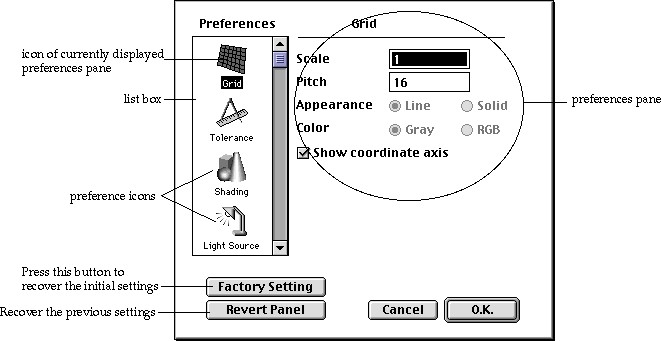
The initial state of the grid is determined by grid settings. To bring up "Grid" pane in the preferences dialog, click "Grid" icon in the list box. The pane has the following items:
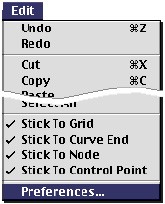
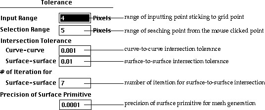
There are tolerances applied for sticking to grid point, selection range and so on. The tolerance can be set on "Tolerance" pane of "Preference" dialog. The pane can brought up by clicking "Tolerance" icon in the list box.
|
"Input Range" If "Ctick to Grid" item in |
||
| "Selection Range" : The nearest object among the front most ones is always selected by a mouse click, when the appropriate selection tool is activated. The selected object need not be exactly on the point of mouse click. There is a tolerance range from the clicked point, within which the nearest object is searched and selected. | ||
| "Intersection Tolerance" : The intersection between curves or between surface primitives are obtained recursively or iteratively. The intersection tolerances set the precision of the recursion or iteration. | ||
|
- "Curve-curve" : tolerance of intersection between curves. |
||
|
- "Surface-surface" : tolerance of intersection between two surface primitives. |
||
| "Number of iteration" : The precision of the intersection is set by the tolerance. On the other hand, there is also a limit in the number of iterations. | ||
|
- "Surface-surface" : The maximum number of iterations is applied only for surface-to surface intersection. |
||
| " Precision of surface primitives : A mesh can be generated on a surface primitive by automatic triangulation. The nodal points on the mesh are constrained on the primitive surface up to its precision. | ||
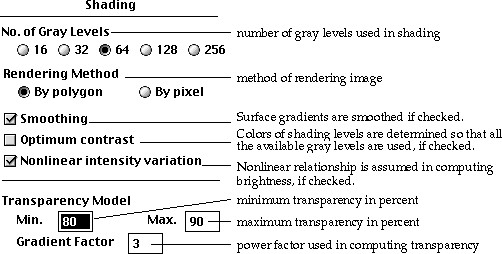
The finite element models are frequently rendered by shading or by contouring with shading. The following options are applied in rendering the models.
| "No. of Gray Levels" : Shading of an object is represented by gray levels. this option determines how many gray levels are used in shading. This option is also applied to contouring with shading. | ||
| "Rendering Method" : Two methods of rendering are used for shading or contouring in VisualFEA. One is rendering by polygon fill. And the other is by painting pixel by pixel based on "area coherence algorithm." The former is faster, but the latter produces better quality. | ||
| "Smoothing" : Smooth surface shading is obtained by smoothing the surface gradients at the element or surface boundary edges. If this option is checked, the gradients are smoothed. Otherwise, they are not smoothed. | ||
| "Optimum contrast" : If this option is checked, the contrast of the shading is determined so that the available gray levels are used as many as possible. Otherwise, the contrast are constant so that absolute gray levels are used for a given shading level. | ||
| "Nonlinear intensity variation" : If this option is checked, nonlinear relationship between the angle of light source and the brightness is assumed in computing the shading level. Nonlinear variation sharpens the bright spot. | ||
| "Transparency Model" : The transparency of the model is computed by the surface gradient, the volume thickness, and angle of light sources. But, the computation is based on a few factors provided in this option. | ||
| - "Min." : Minimum transparency set for the computation. | ||
| - "Max." : Maximum transparency set for the computation. | ||
| - "Gradient Factor" : Factor of power raised to the surface gradient. The computed transparency is affected by this factor. If this factor is larger, surface gradient has smaller effect on the transparency. | ||
> Light source settings
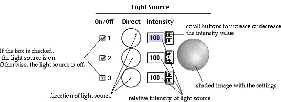
Parallel point light sources are used in shading. There are 3 light sources, with different directions and intensities, each of which can be turned on or off. The light source pane also shows an image of a sphere shaded with the settings.
| "On/off" check boxes: There are 3 check boxes for 3 light sources. If the box is checked, the corresponding light source is on. Otherwise, it is off. | |
| "Direction" circles: The direction of each light source is mapped on a circle, and indicated by a small pointer. The circle re p resents the top view of a hemisphere. The pointer can be dragged to any point within the circle. And the direction of the light source is set accordingly. |
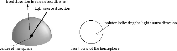
< Mapping of a light source direction >
|
"Intensity" editable text boxes: The relative intensity of each light source can be set in this text box. The values are in percentage. Each intensity value can be inserted by keyboard input or adjusted by using the scroll button on the right of the text box. |
|
| "Immediate Display Mode" check boxes : If this box is checked, the shaded image is updated immediately after the settings are changed. Otherwise, click the shaded image to update the image. |
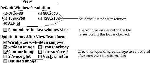
> View settings
View settings control the initial state of the window and the mode of updating the screen contents. The initial width and height of the window are determined by the default window resolution so that the window is sized to fit within the selected resolution. If the default resolution is set to "Actual", the window size is determined based on the actual screen resolution. If "Remember the last window size" box is checked, the size of the window at the time of file saving is restored when the file is opened again. There are several check boxes corresponding to various rendering modes. If the box corresponding to the current rendering mode is checked, the screen contents are redrawn with the rendering mode for every view transformation. Otherwise, the screen contents are updated by wireframe rendering, which produces fastest rendering.
| "Wireframe w/ hidden removal" : Rendering of wireframe with hidden line removal is maintained for every view transformation. | |
| "Shaded image" : Rendering of the model by shading is maintained for every view transformation. | |
| "Transparency" : Rendering of the model by shading with transparency is maintained for every view transformation. | |
| "Contour image" : Scalar data representation by contour image is maintained for every view transformation. | |
| "Iso-surface" : Scalar data representation by iso-surface image is maintained for every view transformation. | |
| "Surface plot" : Scalar data re p resentation by surface plot is maintained for every view transformation. | |
| "Vector image" : Vector data representation by arrow image is maintained for every view transformation. | |
| "Outline image" : Rendering of the model by outline is maintained for every view transformation. |
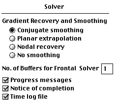
> Solver settings
Solversettings have several options applied during the solution process. These options are applied as defaults for subsequent finite element analysis. "Solver" pane can brought up by clicking "Solver" icon in the list box.
|
|
|
|