![]()
| Data Assignment > Load Conditions > Defining load condition sets for dynamic analysis |
|
|
|
|
||
Defining load condition sets for dynamic analysis
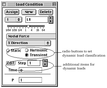
For dynamic analysis, load conditions may or may not have time dependent characteristics. Therefore, assignment of dynamic load conditions involves more steps than that of static load conditions, as described below.
> Setting the time dependency
The dynamic load condition is classified further its time dependency as follows.
|
static: static load condition independent of time. |
|
|
harmonic: time-dependent load condition with periodically changing magnitude expressed by a sinusoidal equation. |
|
| transient: time-dependent load condition represented in multiple time steps. Thus, "Load Condition" dialog for dynamic analysis has radio buttons, "Static", "Harmonic" and "Transient." Time dependency of a dynamic load is set by turning on the corresponding radio button on "Load Condition" dialog. As you alter the time dependency, you will notice the changing items below the radio buttons. Time dependent attributes of dynamic loads are defined and modified using these items. |
> Defining static load for dynamic analysis
Static load condition is assumed to have constant magnitude, direction and position throughout the whole duration of analysis, and can be defined and assigned in the same way as for static analysis. "Static" radio button should be turned on to start defining static loads.
> Defining harmonic load for dynamic analysis
A harmonic load has periodic characteristics with changing magnitude expressed by the sinusoidal function . The intensity of the load acting at a sin specific time is obtained by multiplying the function by the constant load intensity given at the bottom of the dialog.

> Defining transient load for dynamic analysis
A transient load is defined by a series of values at a number of time steps, which can be created and edited by the following steps.

< An example of transient load>
The data on the last line are assumed to be maintained up to the last time step in the analysis. Thus the data shown in the above example dialog will create the following time series data.
|
|
|
|