![]()
| Postprocessing of Continuum Analysis > Visualizing Scalar Data by Iso-surface and others > Curve plotting of scalar data |
|
|
|
|
||
Curve plotting of scalar data
 |
Curve plotting is a method of re p resenting the data distribution along a specified line in the form of graph. This method is supplementary to contouring, and should be preceded by contouring. Curve plotting converts a contour image into graphical representation. The data values along a specified line are extracted and plotted in the form of graph, which gives, in some cases, more descriptive and more detailed information than contour lines do. Curve plotting can be applied to contour images on any plane or surface including cut plane and parallel planes. Numerical data can also be viewed using the curve plotting. This function is available for both 2-D surfaces and 3-D volumes. |

< Curve plotting >
> Initiating curve plotting
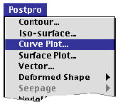
Curve plotting is initiated by choosing "Curve Plot"
item from ![]() menu
. Then, "Curve Plot" window appears on the screen, and
menu
. Then, "Curve Plot" window appears on the screen, and ![]() menu is attached on the menu bar. A bounding box surrounds the model rendered
in the main window, and the initial state of the sampling line is drawn across
the bounding box. The curve plot is displayed on "Curve Plot" window,
for the initial setting. Prior to initiating curve plotting, a contour image
should be displayed. Data of the contour image becomes the subject of the curve
plotting.
menu is attached on the menu bar. A bounding box surrounds the model rendered
in the main window, and the initial state of the sampling line is drawn across
the bounding box. The curve plot is displayed on "Curve Plot" window,
for the initial setting. Prior to initiating curve plotting, a contour image
should be displayed. Data of the contour image becomes the subject of the curve
plotting.
> Modifying curve plotting
At the time curve plotting is initiated, "Curve Plot" window contains a graph representing the magnitude of the data value along the sampling line initially set by the software. This curve plot can be modified or adjusted by further interaction in the main window and "Plot Window" Most importantly, a new plot can be obtained by moving the sampling line. The sampling line can be moved and slanted by using mouse click and drag by the following steps:
|
1) Set the |
|
|
|
|
|
2) Place the screen cursor on one end of the sampling line, and press the mouse button. |
|
|
The color of the sampling line is altered, indicating that the sampling line is selected. |
|
|
3) Drag the end of the line with the mouse button pressed. |
|
|
The end of the line moves along with the cursor, and accordingly the position and the direction of the line are changed. The graph on "Curve Plot" window is updated as soon as the sampling line is modified. |
|
|
4) Double click an edge of the bounding box to change the direction of the sampling line quickly. |
|
|
Double clicking an edge of the bounding box induces one end of the sampling line positioned on the center of the edge, and the other end on the center of the opposite edge. |
> Displaying the numerical value at the sampling point
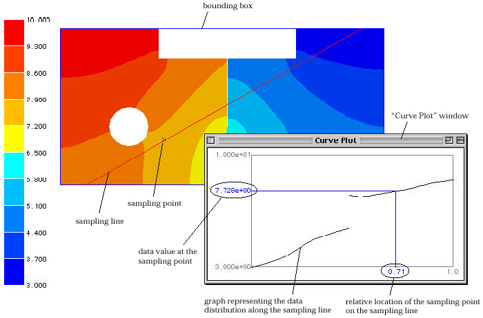
A point on the sampling line can be designated as the sampling point. Click one point on the sampling line. Then, the sampling point is set at the point, and indicated by mark. The numerical value of the data on the sampling point is displayed in a character string on "Curve Plot" window. The relative location of the sampling point over the sampling line is indicated by hair lines and a character string on "Curve Plot" window as shown in the above figure. The sampling point can be moved along the sampling line interactively by using mouse drag. While the point is being moved, the numerical value is updated continuously together with the mark of the newly positioned point.
> Resizing the graph
The graph is drawn to fit the plotting window. Thus, the size of the graph can be changed by resizing the window. Click the bottom right corner of the window, and drag. Or, click the zoom box of the window. Then the graph is resized to fit the new window frame.
> Setting the options for curve plotting
When curve plotting is initiated, ![]() menu appears on the menu bar. The menu has items related to controlling the
sampling line and updating "Curve Plot" window.
menu appears on the menu bar. The menu has items related to controlling the
sampling line and updating "Curve Plot" window.
> Terminating curve plotting
Curve plotting is terminated by clicking the close box at the top left corner
of the "Curve Plot" window, or by initiating any other function. The
bounding box and the sampling line disappear from the main window at the moment
the "Curve Plot" window goes away. ![]() menu also disappears from the menu bar.
menu also disappears from the menu bar.
|
|
|
|